
New Titan Valve
Small Size. Outstanding Performance.
Designed and tested to ensure reproducible, precise, low-pressure fluidic distribution.

Explore SearchLight
Free Spectral Analysis Tool
Discover 6 simple tips and tricks featuring a few of SearchLight’s many capabilities to help you simulate optical filters, search our catalog, and visualize data.

New Rapid Prototype Valve Program
Partner With Us
We can accelerate your instrument development and deliver on time.

New Melles Griot
XPLAN™ CCG Lens Series
Accelerate your Life Science instrument development process. Featuring off-the-shelf lead time with custom design performance.

Semrock Resources
Looking for more info about Semrock?
Learn more about our optical filter capabilities, find sets by fluorophore, download our 2023 Semrock catalog and more.
You See Innovation, We See Your Roadmap
We are component and system-level experts who understand the critical inter-dependencies between fluidics, optics, microfluidics, and integrated sub-assemblies. We specialize in the complete optofluidic pathway to help you avoid project risks and are uniquely positioned to solve even the most demanding challenges in a wide array of applications.
Column Hardware
Explore our extensive line of HPLC and UHPLC column hardware optimized to enable selectivity, efficiency, and high-quality separation performance in your flow paths.
Degassers
Explore our broad portfolio of vacuum degassing assemblies to control bubbles in a wide range of system-fluids and flow-rates.
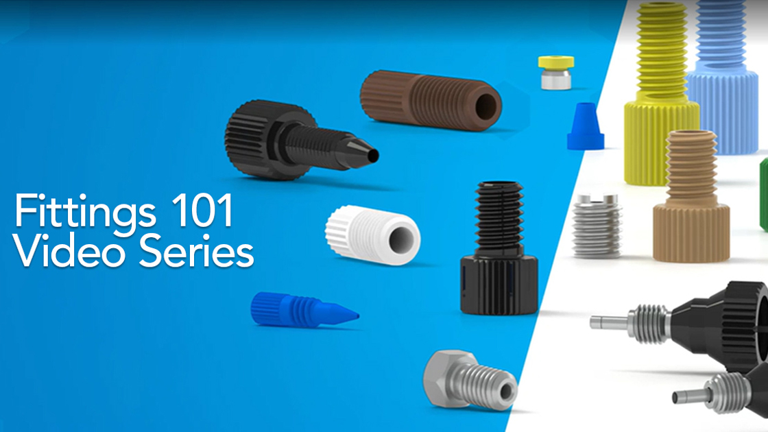
Fluidic Connections
Explore our comprehensive line of tubing, connectors, fittings, and flow control devices that meet the increasingly demanding requirements of today’s high performance analytical fluidic systems.
Pumps
Explore our long-life precision dispense pumps designed for use in a range of clinical and laboratory instruments.
Sensors
Accurately monitor and control your pressure to achieve accurate instrument output and maximized system capabilities with our sensors.
RI Detectors
Achieve high resolution and low dispersion detection with our RI detectors for HPLC applications.
Valves
Explore manual valves for lower frequency use, rotary shear valves that meet the high duty cycle requirements of UHPLC, and more
Individual Filters
Select your bandpass, edge filters, dichroics, and more by key fluorophores.
Optical Filter Sets
Explore single-band and multi-band sets for popular applications and wavelengths.
Shop by Fluorophore
Looking for a filter set to go with your fluorophore? Use the chart on this page to find which Semrock optical filter sets are compatible with popular fluorophores.
Discontinued Semrock Optical Filter Products
Our products are regularly revised to improve performance. Find replacement products here.
SearchLight
Select the elements of your fluorescence system and quickly calculate a relative signal brightness, autofluorescence level, and signal to noise ratio.
Optical System Design
Partner with our optical design and engineering experts to build a fully integrated system for your instrument.
Illumination Solutions
Explore a wide range of laser and LED illumination light engines to meet your application needs from Next Generation Sequencing, Cytometry, Fluorescence Microscopy, and Spectroscopy in clinical and research environments.
Custom Microscope Objective
Partner with our optical design and engineering experts to build a custom objective solution optimized for high-NA, wide field of view, and diffraction-limited resolution performance.
CMOS and CCD Cameras
Looking to replace your CCD camera and achieve similar performance? Consider an IDEX Health & Science CMOS camera with higher resolution and throughput.
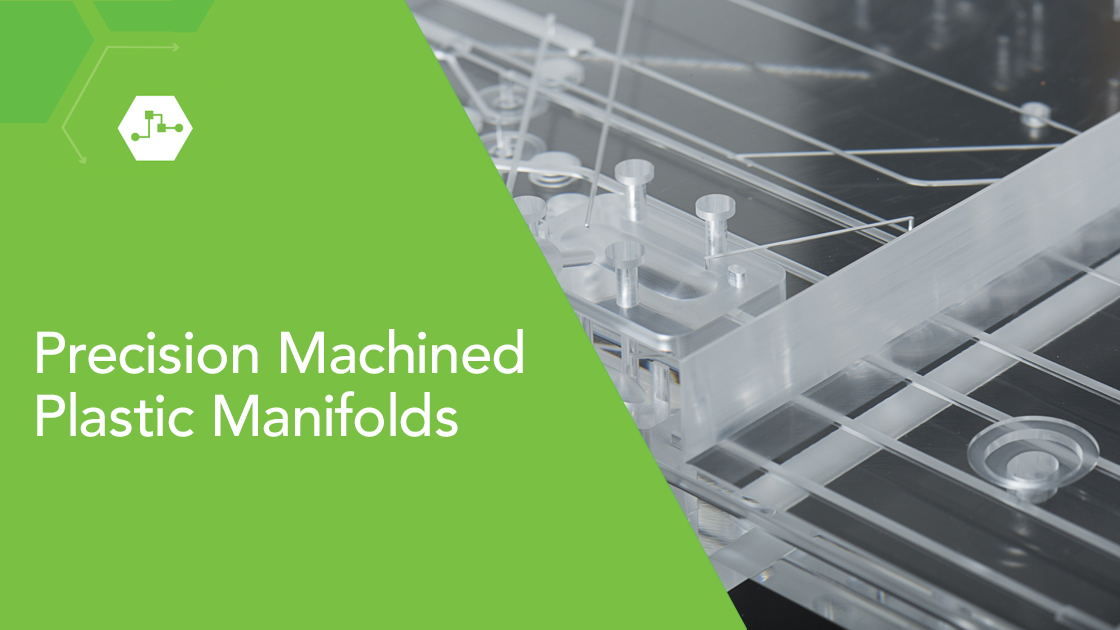
Fluidic Subsystems
Challenged with minimizing expensive reagent volumes while maintaining a cost effective, reliable platform? Partner with our fluidic design and engineering experts to manufacture subsystem solutions to mitigate risk to performance and minimize cost.
Custom Fluidic Solutions
Enhancing reliability, preventing leakage, minimizing carryover, and enhancing usability. These are a few of the many advantages in partnering with us for custom fluidic solutions.
We believe partnership will change the way the world innovates, leading to new technologies that improve our health, protect our planet, and enrich our lives.
The Key to the Future is Collaboration
Watch the below videos to discover how IDEX Health & Science partners with industry experts to change the way the world innovates. We help design and manufacture new technologies that improve our health, protect our planet, and enrich our lives.
About Us
We are the global leader in life science fluidics, microfluidics, and optics, offering a three-fold advantage to customers by bringing optofluidic paths to life with strategic partnerships, solutions, and expertise. As one of the few companies in the world with component, sub-system, and application level experts, IDEX Health & Science helps instrument developers solve the most demanding fluidic and optical challenges in a wide array of applications.
News

IDEX Health & Science is the global authority in fluidics and optics, bringing to life advanced optofluidic technologies with our products, people, and engineering expertise. Intelligent solutions for life.